Showing posts with label Data Structure. Show all posts

Tuesday, 10 February 2015

Sorting

Sorting
Sorting is the process of placing elements from a collection in some kind of order. For example, a list of words could be sorted alphabetically or by length. A list of cities could be sorted by population, by area, or by zip code. We have already seen a number of algorithms that were able to benefit from having a sorted list (recall the final anagram example and the binary search).

Types of sorting algorithms –
1.Bubble Sort
2.Selection Sort
3.Insertion Sort
4.Quick Sort
5.Merge Sort
6.Heap Sort
7.Radix Sort
8. Shell Sort etc.

Internal and External Sorting

ØInternal sort is any data sorting process that takes place entirely within the main memory of a computer.
This is possible whenever the data to be sorted is small enough to all be held in the main memory.
ØExternal sorting is a term for a class of sorting algorithms that can handle massive amounts of data.
External sorting is required when the data being sorted do not fit into the main memory of a computing device (usually RAM) and instead they must reside in the slower external memory (usually a hard drive). 
External merge sort
One example of external sorting is the external merge sort algorithm, which sorts chunks that each fit in RAM, then merges the sorted chunks together.
For example, for sorting 900 megabytes of data using only 100 megabytes of RAM

Bubble Sort

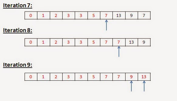
The simplest sorting algorithm is bubble sort. The bubble sort works by iterating down an array to be sorted from the first element to the last, comparing each pair of elements and switching their positions if necessary. This process is repeated as many times as necessary, until the array is sorted. Since the worst case scenario is that the array is in reverse order, and that the first element in sorted array is the last element in the starting array, the most exchanges that will be necessary is equal to the length of the array. 

Ø Move from left to right end
Ø    Compare the two elements and swap them if needed


Algorithm Bubble_sort(a,n): This algorithm sort the elements in ascending order. a is linear array which contains n elements. Variable temp is used to facilitate the swapping of two values. I and J are used as loop control variables.

Analysis of Bubble Sort (version 1) :
For Step 2 :
I =1  J= 0 to (n-2) i.e. total (n-1) and 1 for false. Hence n times
I =2   J =0 to (n-3) i.e. total (n-2) and 1 for false. Hence n-1 times
…….
I=n-1  J=0 to (n-1-n+1) i.e. total 1 and 1 for false. Hence 2 times.

Time Complexity   = n * C1 + {n(n+1)/2 – 1}* C2 + {n(n+1)/2 – 2}* (C3+C4+C5+C6)
  = n + (n2 + n - 2) /2 + 2*(n2 + n - 4)
  = O(n2
Analysis of Bubble Sort (version 2) :
From the above illustration, we observe following points –
In (n-1) iterations or passes array will become sorted.
Iteration 1:   no. of comparisons (n-1)
Iteration 2:   no. of comparisons (n-2)
Iteration 3:   no. of comparisons (n-3)
………………..
Iteration k:   no. of comparisons (n-k)
……………...
Iteration last:   no. of comparisons 1
Time Complexity   = Total Comparisons
  = (n-1) + (n-2) + (n-3) + ….+ (n-k) + …. + 3 + 2 + 1
  = n(n-1)/2
  = O(n2)

Selection Sort
Ø Move from left to right end
Ø    Each time least element gets its final position i.e. we select least element and put it at it’s final position


Algorithm Select_sort(a,n): This algorithm sort the elements in ascending order. a is linear array which contains n elements. Variable temp is used to facilitate the swapping of two values. I and J are used as loop control variables.
1.For I = 0 to n-2 
2.       For J = I+1 to (n-1)
3.                    If a[I] > a[J] then,
4.                             Set temp = a[I]
5.                             Set a[I] = a[J]
6.                             Set a[J] = temp 

Analysis of Selection Sort

From the above illustration, we observe following points –
In (n-1) iterations or passes array will become sorted.
Iteration 1:   no. of comparisons (n-1)
Iteration 2:   no. of comparisons (n-2)
Iteration 3:   no. of comparisons (n-3)
………………..
Iteration k:   no. of comparisons (n-k)
……………...
Iteration last:   no. of comparisons 1
Time Complexity   = Total Comparisons
  = (n-1) + (n-2) + (n-3) + ….+ (n-k) + …. + 3 + 2 + 1
  = n(n-1)/2
  = O(n2)


Monday, 9 February 2015

Searching Algorithms

Searching
Objective : To find out the location of any given element in array. If element found then successful, otherwise unsuccessful.
Two approaches –

1.Linear Search (Sequential Search): if array elements in random order

2.Binary Search: if array elements in sorted order

Linear Search

Algorithm: Let a is given array and no. of elements is n. Pos is representing the position of desired element k in array a, if element found otherwise, set Pos to -1. Variable i is used as simple variable in loop. 

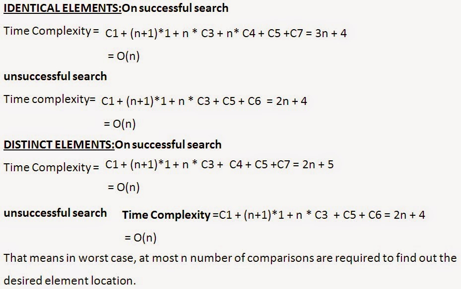
Analysis of Linear Search


Binary Search

Ø    Best searching approach
Constraint:
§  Given array should be in sorted order
  OR
§  First sort the given array and then perform search, but then sorting time will be   added

Binary Search (Iterative)

Algorithm: Let a is given array which is sorted in ascending order and no. of elements is n. Pos is representing the position of desired element Item in array a, if element found otherwise, set Pos to -1. Variable mid is used to keep the mid index of array.

1.Initialize low =0, high = n-1
2.While low <= high
3.       mid =    (low+high)/2
4.       If a[mid] == Item
5.                    Set Pos = mid
6.                    Break and Jump to step 10
7.       Else if Item < a[mid]
8.                     high = mid -1
9.       Else   low =mid +1
10.If Pos < 0
11.        Print “Element is not found”
12.Else  Print Pos

Binary Search Illustration


Binary Search (Iterative)


Analysis of Iterative Binary Search


Binary Search (Recursive)

Algorithm Bin_Search(a, Item,low, high): Let a is given array which is sorted in ascending order and no. of elements is n. Pos is representing the position of desired element Item in array a, if element found otherwise, set Pos to -1. Variable mid is used to keep the mid index of array. Here, initially low and high are assigned the lowest and highest index of array a.
1.If low<=high
2.         mid =    (low+high)/2
3.         If a[mid] == Item
4.                        Set Pos = mid
5.                         Return Pos
6.         Else if Item < a[mid]
7.                         Return Bin_Search(a,Item,low,mid-1) 
8.         Else        Return Bin_Search(a,Item,mid+1,high)
9.Return Pos

Problem

For the code segment below estimate the time-complexity in the big-oh notation.
for (int i=0; i< n; i++)
         for (int j=0; j*j <n;j++)
                    for (int k=0; k < n/2;k++)
                                print (i+j+k);
Soln:
Loop 1 rate of change depends linearly on n -> O(n) -- Linear
Loop 2 rate of change depends on the squared root of n -> O(n^0.5) -- Fractional power
Loop 3 rate of change depends linearly on n/2, but 1/2 constant can be removed -> O(n/2) -- Linear
So, the overall complexity would be O(n) * O (n^0.5) * O (n) = O (n^2.5)

Complexity analysis of an algorithm

Two main methods:
1.Direct counting:Time complexity will be sum of the individual steps (primitive Operations)
Best for repeated iterations (loops).
2.      Recurrence equation(Recurrence Relations):
an equality or inequality describing the function in terms of its behavior on smaller inputs.
Best for recursive functions and structures.

Recurrence Relation  


Base Case:
When you write a recurrence relation you must write two equations:
one for the general case and
one for the base case.
These correspond to the recursive function to which the recurrence applies. The base case is often an O(1) operation, though it can be otherwise.
In some recurrence relations the base case involves input of size one, so we wrote 
T(1) = O(1).
However, there are cases when the base case has size zero. In such cases the base could would be 
T(0) = O(1). 


Solving Recurrence Relations
T(n) = 2 T(n/2) + O(n)       // [the O(n) is for Combine]
T(1) = O(1)                         // Base Case
We'll write n instead of O(n) in the first line below because it makes the algebra much simpler.
T(n) = 2 T(n/2) + n
= 2 [2 T(n/4) + n/2] + n
= 4 T(n/4) + 2n
= 4 [2 T(n/8) + n/4] + 2n
= 8 T(n/8) + 3n
=16 T(n/16) + 4n
…..
…..
= 2k T(n/2k) + k n
We know that T(1) = 1 and this is a way to end the derivation above.
In particular we want T(1) to appear on the right hand side of the = sign.
This means we want:
n/2k = 1 OR n = 2k OR log2 n = k
Continuing with the previous derivation we get the following since k = log2 n:
= 2k T(n/2k) + k n
= 2log2 n T(1) + (log2n) n = n + n log2 n
= O(n log n)
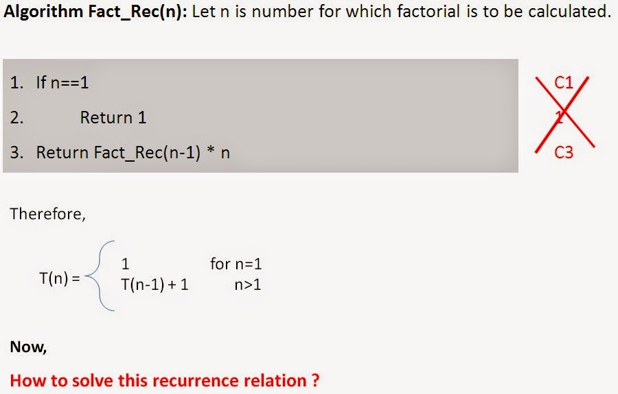
Illustration 1: Factorial Recursive 

Substitution method – try to find the pattern
While the equation certainly expresses the complexity function, a non-recursive (or closed-form) version would be more useful.
T(1) = 1
T(n) = T(n -1) + 1
T(n) = T(n -1) + 1   //T(n - 1) = T(n - 2) + 1
= T(n - 2) + 1 + 1
= T(n - 2) + 2  //T(n - 2) = T(n - 3) + 1
= T(n - 3) + 1 + 2
= T(n - 3) + 3   //T(n - 3) = T(n - 4) + 1
= T(n - 4) + 4
= : : :
= T(n - k) + k
If we set n-k=1=> k=n-1 we have:
T(n) = T(1) + n-1
= 1+n-1
T(n)= n
Hence, Time complexity = O(n)
Illustration 2: Fibonacci Recursive


This the case of Deep recursion where if the function makes more than one call to itself, you have a deep recursion, that takes exponential time.
Ø   It grows like exponential tree.
Time complexity = O(2n)

Analysis of Binary Search Recursive


T(n)   = T(n/2) + 1
  = T(n/2*2) + 1 + 1
  = T(n/2*2*2) + 3
  = T(n/24) + 4
  …………….
  = T(n/2k) + k
Let    n/2k = 1,   n = 2k ,   log2n = k * log22
i.e.      k = log2n
Now,
  T(n)  = T(1) + log2n = 1 + log2n
  = O(log2n)

Recurrence Relations to Remember